はじめに
3Dスキャンデータを処理する際、異なる視点から取得した点群データを統合する場合があります。その際に役立つのが ICP(Iterative Closest Point) です。本記事では、PythonとOpen3D を使用して、ICPを実装する方法を解説します。
ICPとは?
ICP(Iterative Closest Point)は、Besl and McKay (1992) によって提案されたアルゴリズムで、2つの点群を最適に位置合わせするために用いられます。
ICPの基本手順
- 各点群間で最も近い点のペアを見つける
- 点の対応関係から最適な剛体変換(回転 + 並進)を求める
- 点群を変換し、誤差が収束するまで繰り返す
このアルゴリズムの詳細については、以下の論文を参照してください。
- P. Besl and N. McKay, “A Method for Registration of 3-D Shapes,” IEEE Transactions on Pattern Analysis and Machine Intelligence, vol. 14, no. 2, pp. 239-256, 1992. DOI: 10.1109/34.121791
- Zhang, Z. “Iterative point matching for registration of free-form curves and surfaces,” International journal of computer vision, vol. 13, pp. 119-152, 1994.
後述するサンプルコードでも解説しますが、実行したいことは「基準点群に対して、参照用点群を一致させる」です。
よって、基準点群に対して参照用点群を位置的に一致させるような同次変換行列(回転と並進を操作可能な4×4行列)を導出することがIPCのゴールになります。
同次変換行列については以下の記事を参照ください。
(後日執筆予定)
ICPの活用例
ICPはさまざまな分野で活用されています。例えば、ロボットの自己位置推定(SLAM) において重要な役割を果たします。
SLAM(Simultaneous Localization and Mapping)は、ロボットが未知の環境を探索しながら地図を作成し、自身の位置を特定する技術です。SLAMの過程でロボットは、LiDAR(レーザースキャナー)やRGB-Dカメラを用いて取得した点群を統合する必要があります。この際、各フレーム間の点群を位置合わせするためにICPが使用されます。
例えば、
- 自動運転車の環境認識
- ドローンによる3Dマッピング
- 倉庫ロボットのナビゲーション
といった用途で、ICPが重要な役割を担っています。
実行環境
本記事の実行環境です
- OS:Windows 10
- Python Ver.3.11
- Open3d Ver.0.18.0
インストールはこちらを参考にしました。
処理対象の点群および課題設定
処理対象の点群
RealSenseにより取得した2種類の点群およびテキスチャ情報を処理対象とします。
(データ取得はこちらのコードを使用)
- realsensebox_leftangle.ply
- 参照用点群:赤色
- RealSenseの箱を左斜め上から撮影したもの
- realsensebox_rightangle.ply
- 基準点群:緑色
- RealSenseの箱を右斜め上から撮影したもの
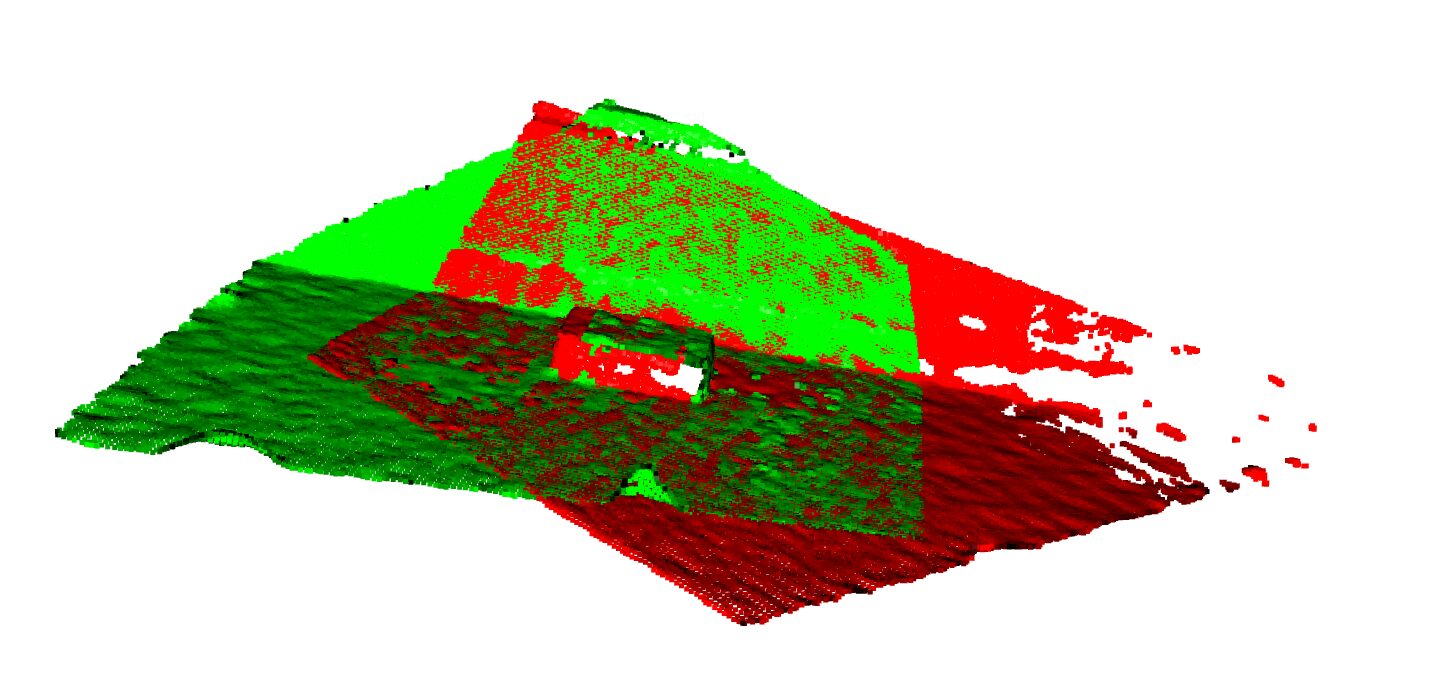
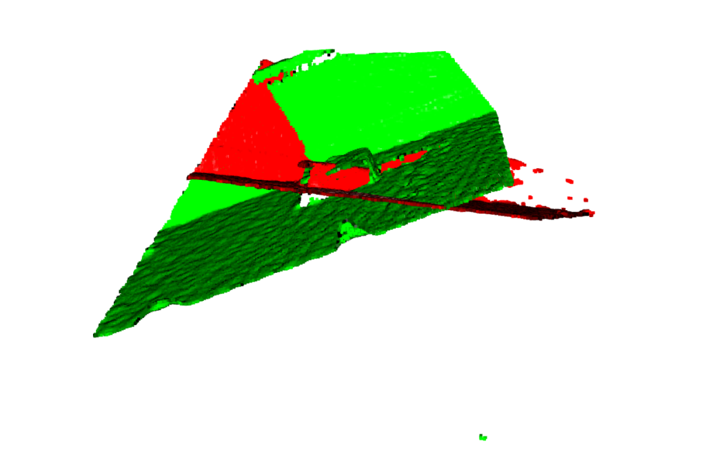
両方の点群を表示すると以下のようになります。
赤が「realsensebox_leftangle.ply」、赤が「realsensebox_rightangle.ply」
課題設定
ICPの適用により、二種類の点群の位置合わせを行う。
ICPの実装
サンプルコード
import open3d as o3d
import numpy as np

# PLYファイルを読み込む
# ファイルは別視点から取得した点群データを用意してください。
source = o3d.io.read_point_cloud("icp/realsensebox_leftangle.ply")  # 参照用点群
target = o3d.io.read_point_cloud("icp/realsensebox_rightangle.ply")  # 基準点群

# 外れ値除去
source = source.remove_statistical_outlier(nb_neighbors=20, std_ratio=2.0)[0]
target = target.remove_statistical_outlier(nb_neighbors=20, std_ratio=2.0)[0]

# ダウンサンプリング
source = source.voxel_down_sample(voxel_size=0.005)
target = target.voxel_down_sample(voxel_size=0.005)

# 変換後の点群を可視化
source.paint_uniform_color([1, 0, 0])  # 赤
target.paint_uniform_color([0, 1, 0])  # 緑
o3d.visualization.draw_geometries([source, target])


threshold = 0.02  # 近傍探索の閾値
trans_init = np.eye(4)  # 初期変換行列(単位行列)

# ICPの実行
reg_p2p = o3d.pipelines.registration.registration_icp(
    source, target, threshold, trans_init,
    o3d.pipelines.registration.TransformationEstimationPointToPoint(),
    o3d.pipelines.registration.ICPConvergenceCriteria(max_iteration=200)
)

print("ICP変換行列:")
print(reg_p2p.transformation)
# 参照用点群に対して変換行列により剛体変換
source.transform(reg_p2p.transformation)
# 変換後の点群を可視化
o3d.visualization.draw_geometries([source, target])
サンプルコードの深堀り
import open3d as o3d
import numpy as np

# PLYファイルを読み込む
# ファイルは別視点から取得した点群データを用意してください。
source = o3d.io.read_point_cloud("icp/realsensebox_leftangle.ply")  # 参照用点群
target = o3d.io.read_point_cloud("icp/realsensebox_rightangle.ply")  # 基準点群

# 外れ値除去
source = source.remove_statistical_outlier(nb_neighbors=20, std_ratio=2.0)[0]
target = target.remove_statistical_outlier(nb_neighbors=20, std_ratio=2.0)[0]

# ダウンサンプリング
source = source.voxel_down_sample(voxel_size=0.005)
target = target.voxel_down_sample(voxel_size=0.005)

# 点群を可視化
source.paint_uniform_color([1, 0, 0])  # 赤
target.paint_uniform_color([0, 1, 0])  # 緑
o3d.visualization.draw_geometries([source, target])o3d.io.read_point_cloud():PLYやPCDなどの形式の点群データを読み込む関数- 引数
filename (str): 読み込む点群データのファイルパスformat (str, optional): ファイルフォーマット(自動判別)
- 戻り値:
o3d.geometry.PointCloudオブジェクト(点群データ)
- 引数
remove_statistical_outlier():外れ値除去- 引数:
nb_neighbors (int): 近傍点の数std_ratio (float): 外れ値の判定に用いる標準偏差の閾値
- 戻り値:
(filtered_cloud, indices)のタプル(外れ値除去後の点群と、残った点のインデックス)
- 引数:
voxel_down_sample():点群のダウンサンプリングを行う関数- 引数:
voxel_size (float): ボクセルサイズ(単位: メートル)
- 戻り値: ダウンサンプリングされた
o3d.geometry.PointCloudオブジェクト
- 引数:
paint_uniform_color():点群の表示色の変更- 引数:
color (list of float): RGB値(0〜1の範囲)
- 戻り値:
None(点群の色を変更)
- 引数:
o3d.visualization.draw_geometries():点群の可視化- 引数:
geometries (list): 可視化する3Dオブジェクトのリスト
- 戻り値:
None
- 引数:
threshold = 0.02  # 近傍探索の閾値
trans_init = np.eye(4)  # 初期変換行列(単位行列)

# ICPの実行
reg_p2p = o3d.pipelines.registration.registration_icp(
    source, target, threshold, trans_init,
    o3d.pipelines.registration.TransformationEstimationPointToPoint(),
    o3d.pipelines.registration.ICPConvergenceCriteria(max_iteration=200)
)

print("ICP変換行列:")
print(reg_p2p.transformation)
o3d.pipelines.registration.registration_icp:ICPの実行- 引数:
source (PointCloud): 変換対象の点群target (PointCloud): 基準となる点群threshold (float): 対応点探索の最大距離trans_init (np.ndarray): 初期変換行列(4×4)
- 戻り値:
reg_p2p(変換行列や一致度の情報を含む)
- 引数:
# 参照用点群に対して同次変換行列を適用
source.transform(reg_p2p.transformation)
# 変換後の点群を可視化
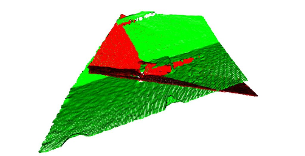
o3d.visualization.draw_geometries([source, target])参照用点群に対して同次変換行列を適用し、基準点群に対して位置合わせを行います。
transform()- 引数:
transformation (np.ndarray): 4×4の変換行列
- 戻り値:
None(点群の座標を更新)
- 引数:

床の平面と床と垂直にある壁、床に設置されたRealSenseの箱が位置合わせされてることがわかります。
まとめ
本記事では、PythonとOpen3Dを使用してICPを実行する方法 を解説しました。
同次変換行列を導出することで、参照用点群を基準点群に対して位置合わせを行うことが可能となりました。
三次元点群処理は二次元の画像処理よりも情報が少なく、手探りで書籍や論文、公式ドキュメントを調査する日々です。
その中で、導入しやすいPythonとOpen3Dで三次元点群処理を体系的にまとめた書籍が以下になります。現在数少ない三次元点群処理の書籍ですので私も重宝しています。是非参考にしてみてください。
参考リンク
社内外で評価されるエンジニアになる、ひいてはエンジニア人生を楽しくするためには、
日常のインプットとアウトプットの重要性が日に日に増していることを実感しています。
そのなかで、私は「書籍による学習」と「ブログによるアウトプット」を強くおすすめしております。
その重要性や効果の実感をブログに書いてみましたので、参考にしていただければ幸いです。